


Investing Strategy: Improving my DCF model
Taking Michael Mauboussin's advice on board

A couple of months ago, Summit Stocks posted a summary of an article written by Michael Mauboussin1 in 20062, about errors typically seen in Discounted Cash Flow (DCF) models. It’s a fascinating read, that I highly recommend. I’ve embedded the link at the bottom of this post.
Without replicating either the original article by Mauboussin, or the summary by Summit Stocks, the main errors Mauboussin highlights are:
Forecast horizon is too short. Evidenced by the terminal value contributing a large proportion of the total corporate value (Mauboussin states 60% - 70%), and results in a typically low valuation. Mauboussin also points out that if investors are willing to pay 20 - 30 times earnings for a stock, then they should be willing to estimate earnings for that period (as that’s the time it would theoretically take to return an investment in terms of growth in corporate value (retained earnings) in the absence of re-investment or growth).
Uneconomic continuing value. In other words, considering an unrealistic return on capital in perpetuity. Mauboussin uses the example of an assumed multiple implying returns on capital that are unrealistically excessive.
Cost of Capital estimates. Mauboussin suggests the use of the Capital Asset Pricing Model (CAPM) for cost of equity is an imperfect theoretical underpinning (but he doesn’t offer an alternative).
Mismatch between assumed investment and earnings growth. That is, models not reflecting the reality that it becomes progressively harder and more expensive to continue to grow earnings as a company becomes more mature.
Improper reflection of other liabilities. The specific example chosen by Mauboussin is employee stock options, suggesting that fully-diluted shares is a poor reflection of options and contingent liabilities.
Discount to private market value. That is, the lack of marking to market for private companies.
Double-accounting. For example, assuming share buybacks in addition to free cash flow generation, yet it is the same free cash flow that is used to enable the share buyback.
Scenarios. In other words, not considering multiple scenarios when trying to assess value.
While I don’t believe I need to consider all of these errors, and I already address some errors through my Monte Carlo approach, a number of these concerns chimed with me, as I knew my modelling approach was weak in a number of these areas. So I took some time to think about and update my models.
Re-assessing my DCF model
Comparing my modelling approach to the points raised by Michael Mauboussin, I draw the following conclusions:
Forecast horizon is too short. I definitely feel this applies to me. I use a 5 year forecast period (explicitly referenced by Mauboussin as being the minimum period) because I don’t want to project too far into the future, which is obviously inherently uncertain. But the consequence is that my valuations are often below market value, especially for high-growing companies, and the terminal value of my models is often a high percentage of the total value.
Uneconomic continuing value. I use the Gordon Growth Model for my terminal value assessment, limited by a maximum P/E multiple. Therefore I may be susceptible to this error when my cost of capital estimate is very close to my perpetual growth rate.
Cost of Capital estimates. This definitely applies to me because I use the CAPM model for my cost of equity, but because I consider variation in that cost of equity, the sensitivity of my model to beta is implicit. I have often thought about replacing beta in my cost of equity model with a more appropriate downside risk metric, maybe something like the Sortino Ratio.
Mismatch between assumed investment and earnings growth. Another error that definitely applies to my modelling approach, as I assume an explicit and independent earnings growth rate and free cash flow growth rate, meaning I have the ability to estimate a lower (or higher) growth in free cash flow compared to earnings, but I don’t use this flexibility to link free cash flow to investment, or investment to earnings.
Improper reflection of other liabilities. Another error that applies to me, but I also tend not to value companies with complicated liabilities or stock options, so I don’t know that I need to worry too much about this error currently. However, I do use fully-diluted share count when assessing value.
Discount to private market value. I tend not to value private companies, but when I do (for example, in the case of an acquisition or a company coming to IPO), I don’t apply any kind of premium, so I don’t think this applies to me.
Double-accounting. This doesn’t fully apply to me - I don’t assume any reduction in share count in addition to free cash flow generation. I am assessing a present value, based on the present share count. However, I do subtract interest expense when assessing operating cash flow and I do consider book value, by which I am deducting total debt (and other liabilities) from total assets. This feels like an example of the double-accounting Mauboussin mentions (you either pay off the debt or you pay the debt interest expense, you don’t do both), so I may need to reconsider the book value used in my models. However, this level of double-accounting provides some margin of safety (it will tend to reduce valuation, rather than increase it).
Scenarios. Thankfully, another error that doesn’t apply to me. I use Monte Carlo methods in my valuations, meaning I am already considering a range in inputs and assessing a range of results. This also implicitly allows me address some of the other errors e.g. although I don’t explicitly link cost of capital to earnings or free cash flow growth, I may capture the effect as my model will consider scenarios with higher cost of capital in conjunction with lower growth rates, and vice versa (as well as higher cost of capital providing for higher growth rates).
Adjusting my Model
Taking the above points on board, I can see a few obvious areas where I could improve my modelling. Specifically, the forecast period and linking cost of capital to earnings growth and returns. I have also made a modification to the terminal value estimate to rely less often on a multiples approach.
Although this means I am still susceptible to errors with double-accounting for debt, possibly using a multiples approach for terminal value in some specific scenarios, using the CAPM model for cost of equity and not fully accounting for all liabilities, I equally don’t want to change too much in my model at once. I may return to some of these remaining errors as I become more comfortable with my revised model.
The Forecast Period
I had originally set up my model to use an average growth rate (using a geometric average, not an arithmetic average) over a 5 year period, then assuming perpetual growth at the risk-free rate. With this set-up, it isn’t that hard to simply extend the forecast period to 10 years. But should the growth rate then abruptly change to the risk-free rate? The conceptual corporate life cycle implies a gradually declining growth rate until the perpetual growth rate is reached (which I assume to be equal to the risk-free rate). However, as growth in the distant future is heavily discounted to present value, it’s not obvious how much of a difference extending the growth runway will make.
I have therefore set up my model to undertake discounted cash flows over 3 different time periods - my original 5-year period; a new 10-year period (which is a common period used in DCF models); and a 10-year average-growth period with a further 20-year S-curve growth rate, to adjust the growth rate from my assumed average rate used for the first 10 years of the DCF period to the risk-free rate by the end of the S-curve period. In this way, the S-curve approach provides for a 30-year DCF period in total.
To generate the S-curve, I use the following equation (mathematically, the logistic function):
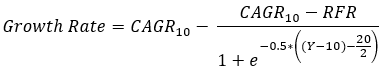
where:
CAGR_10 = compounded annualised growth rate (CAGR) to be used for the first 10 years of the DCF period
RFR = Risk-free Rate, to be used by the end of the 30-year period
Y = the year of the DCF period, from Year 11 to Year 30
the 0.5 parameter and 20/2 parameter are set arbitrarily to scale the equation for a gradual change from the original assumed growth rate to the final risk-free rate over 20 years.
Linking re-investment to earnings growth
In the referenced article, Mauboussin sets out some equations in the Appendix of the article to link Return on Incremental Invested Capital (ROIIC) to growth. I have applied a similar logic, but with some modifications. Return on Invested Capital requires calculation of Net Operating Profit after Tax (NOPAT) and requires an estimate for the amount of earnings re-invested in capital assets. I prefer to use the slightly broader-based Return on Capital Employed (ROCE) instead of ROIC (or ROIIC). ROCE uses Earnings Before Interest and Taxes (EBIT) instead of NOPAT, and Capital Employed does not require as much explicit estimation as Invested Capital. EBIT is commonly quoted and readily available (or can be approximated with operating profit), so is easier to assess than generating specific calculations for invested capital for each stock to be analysed.
My approach starts with an initial estimate for ROCE, which is used for the calculations of the first year of earnings. To adjust between earnings and EBIT, I assume the effective tax rate and use an assumed Cost of Debt on the total debt held by the company. I assume the absolute debt interest payments are unchanged throughout the DCF period, which is likely to be a simplification, as in reality debt is either paid down or renewed at prevailing interest rates. I assume the effective tax rate is also unchanged, but the absolute tax paid will vary as earnings change over the DCF period.
For all subsequent years within my DCF, I assume the capital employed is increased by the prior year’s retained earnings. I assume dividends are paid at a constant percentage of earnings, so retained earnings are equal to last year’s earnings multiplied by (1 - dividend payout ratio). I then recalculate ROCE as that year’s EBIT, divided by the new level of capital employed. I limit the minimum ROCE to the Weighted Average Cost of Capital (WACC), which is itself linked to assumptions I make for cost of debt and cost of equity.
I still use CAPM for cost of equity, but whereas in my original, simple, model I assume the cost of equity is an explicit and independent parameter in my DCF model inputs, now I make explicit assumptions for the stock’s “beta” parameter, the risk-free rate and the market premium, and let CAPM calculate the cost of equity. I then calculate WACC with this cost of equity and my assumed cost of debt.
To calculate earnings and EBIT for each year within the DCF period, I assume a CAGR for revenue growth at a constant EBITDA margin, in conjunction with the effective tax rate and interest payments. I assume depreciation and amortisation (D&A) expenses as a proportion of sales, thereby linking them to EBITDA margins and allowing simple estimation of EBIT margin.
In this way, I can link assumed revenue growth to EBIT, earnings and ROCE. It still isn’t a perfect approximation, as I don’t link ROCE to subsequent revenue growth, or permit EBIT margin to vary over time, but this is still an improvement over my simple model.
To give an example of how ROCE now changes with time, see the example generated below, showing the minimum, lower quartile, upper quartile and maximum ROCE values calculated each year, compared to WACC (the final column). This is characteristic of a corporate life cycle (this specific example was generated using Caterpillar’s 2024 annual report data). What’s also interesting to me, is that the results become more consistent after 10 years, broadly flattening out by years 15 - 20. This also supports Mauboussin’s claim that many DCFs use too short a forecast period, and makes me re-assess my original assumption of using a forecast period of only 5 years.
With this linkage of growth rates to WACC, I no longer require the S-curve logistic function, so in my detailed model I simply use a 30-year forecast period, without any additional approximations to link earnings growth rates to risk-free rates.

Estimating Free Cash Flow
I previously allowed Free Cash Flow to be stated independently of EBIT or earnings, which is not realistic. Now, I take EBITDA as a (crude) approximation of operating cash flow, from which I remove the tax and interest costs. I consider this to be a reasonable approximation of Cash Flow from Operations. I also make an assumption for capital investments as a fraction of sales, and remove that. In this fashion, I am attempting to walk cash flow from operations to free cash flow. This also means I no longer need to estimate free cash flow per share, or estimate free cash flow growth rate - it is inherent to the model, based on assumptions for revenue growth, EBITDA margin, D&A costs and capital investments as a proportion of sales.
Caveats
In a previous job role, I developed engineering models to simulate physical phenomena. I have also previously built statistical parametric models for a number of purposes throughout my working career. I’m going to open with a quote that has served me well professionally:
“All models are wrong, but some are useful” - George Box
Models are, by their very definition, an approximation of the real-world behaviour they are intending to replicate. These approximations mean there are inherent errors, where the model either intentionally or accidentally overlooks certain real-world phenomena, or makes some simplifications for practical purposes or ease of use. This applies to every single model, from detailed mathematical models such as those used in predict weather patterns, to architectural models of new buildings, to Airfix build-it-yourself plane models, to Matchbox car models, to Lego. These models may look like the real product, but they use different materials, don’t have all of the same working mechanisms, etc. However, as long as you are aware of the model’s shortcomings, you can still use it to provideuseful insights (and have fun).
Another quote that I have come across more recently, but that is also very relevant for this discussion, is:
“I’d rather be vaguely right than precisely wrong” - John Maynard Keynes
It is very easy to be over-confident in your model, especially if the model is complex and is capturing many real-world phenomena, as you believe you can trust it in more scenarios than might be wise. When you are extrapolating any model to situations which have not yet occurred, you do not know for sure how well your model will work. Ultimately, if your assumptions for your inputs are wrong, your outputs will likely be wrong (the modeller’s adage: garbage in, garbage out). Often, a simpler and more approximate model can provide better estimates than a very detailed model that may contain more explicit and implicit assumptions.
There is a concept in statistical models related to in-sample and out-of-sample performance, which at a high level reflects how well the model represents the data on which the model was built (in-sample), and how well the model represents performance when fed with data which was not used to build the model (out-of-sample). With enough inputs and enough tuning, it is always possible to create a model that captures historical behaviour accurately, whether or not those input parameters have any true predictive power or not. When building a model, it is good practice to hold back a set of data and then use the model to ‘predict’ performance using that data (as history has already told you what the performance should have been, so you can quantify how well the model reflects an unknown scenario). However, there is a very important parameter missing from any DCF model, and that is investor sentiment - there is no guarantee that that the price of a stock will reflect its intrinsic value at any point in time, now or in the future. For example, most funds trade at a discount or premium to Net Asset Value - you can provide rational hypotheses for why this might be the case, but ultimately a fair value analysis will not capture this phenomenon. The model will always be imperfect.
It is always possible to be right for the wrong reasons. If the model does not have a strong theoretical underpinning, it may still generate what seems to be useful result, either by luck or because the combination of inputs fall within a refined range which obscures the lack of theoretical constraints within the model. The risk comes when you feed the model with input data that seems superficially sensible, but that is not internally coherent, and the model gives you results that could be highly unrealistic (such as extreme values for return on capital, as indicated by Mauboussin). Unless you are alert to this risk, you may take the model results at face value.
For example, my original DCF valuation had no linkage between earnings per share, free cash flow, or average growth rates. It relied on the user to apply sensible values for these parameters, and would blindly present results based on these inputs, irrespective of how realistic it might be to achieve those earnings or free cash flows, independently, in the future. My new model attempts to link future growth to current performance, and to link earnings and free cash flow, so it should not be possible to permit earnings and free cash flow to diverge drastically and grow independently.
Effect of Changes
To put the refined model into practice, I will compare my new outputs to some previously generated results, using my recent valuation of RELX 0.00%↑.
Simple Model - extended forecast periods
I valued RELX in January3 (using the London Stock Exchange listing, LSE:REL). Initially, I will use my simple model with the same inputs, but now incorporate the extended forecast periods. At the time, I estimated the median price for fair value to be £18 - £20, with top-end estimates of £25 - £27.
Re-running the model now, the 5-year forecast period provides median values of £18 - £19, and top-end estimates of £24 - £25. These are similar, but not identical, to what was estimated previously, as expected (the Monte Carlo method I apply means I will always have some inherent variability, even when re-running the exact same model and inputs).
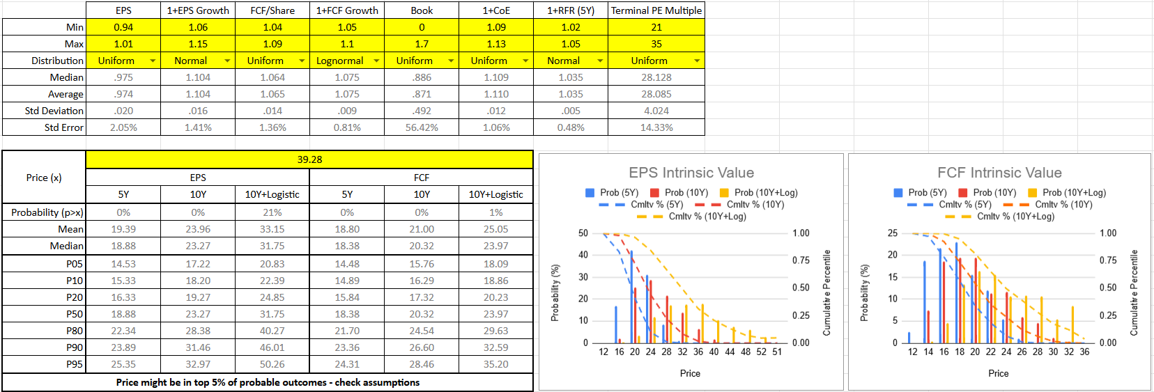
With an increased DCF period, I now estimate the median fair value to be £20 - £23 if the estimated growth rates can be maintained for 10 years instead of just 5 years, with top-end valuations of £28 - £33. If the growth period extends beyond 10 years (relying on my logistic S-curve estimate), I think a median price of up to £24 - £32 could be justified, with top-end estimates of £35 based on free cash flow, or even as high as £50, based on earnings.
This means that extending the DCF period from 5 years to 10 years has increased the price I might be prepared to pay by £2 - £3 at the mid-point, and the top end estimate could be stretched by £5. Extending the growth runway further, up to 30 years (but with a decreasing growth rate) pushes the median value up a further £4 but also increases the range of values that could be considered ‘reasonable’, with a median earnings estimate of £32 now broadly matching the 10-year top-end earnings estimate.
The graphs show that increasing the forecast period tends to spread out the range of possible intrinsic values, making it harder to hone in on a specific value. However, by considering a wider range of possibilities, it also provides more insight into how likely a specific price might be to occur. In this case, the ‘probability (p>x)’ line in Figure 2 indicates that there is a negligible chance that the (then-) current share price of £39 could be justified with either a 5- or 10-year growth period, and that it requires the 30-year growth period to have a chance of justifying the share price. Even then, it is highly unlikely that the price represents fair value based on free cash flow, and it remains fairly unlikely (21%) that the share price can be justified based on future earnings growth. In other words, RELX 0.00%↑ seems like an expensive stock by almost any measure.
Detailed Model
When I use my more detailed model now, I get some more significant differences. As before, with the 5-year forecast period, I estimate a median price of £20 and top-end prices of around £25, so this remains consistent with the simple model. However, now, I estimate a median fair value of around £40 for a 10-year DCF, whether using earnings or free cash flow, vs. £20 - £23 with the simple model. Over a 30-year forecast period, the median fair value could be £42 - £45, vs. £24 - £32 with the simple model. Across the different periods and different valuation metrics, top-end estimates now appear to be between £45 - £55 or even £60, which is a bit higher than the £35 - £50 estimated by the simple model.
For context, the terminal value accounts for roughly 30% +/- 10% of the intrinsic value with a 10-year DCF period, and 20% +/- 10% over a 30-year DCF period. At these levels, the valuation is much, much less sensitive to assumptions around perpetual growth rates, addressing Mauboussin’s criticism of short discount periods.

Suddenly, RELX doesn’t seem so unreasonably priced. Its price can be justified with a 10-year DCF period based on mid-point value estimates. However, as previously discussed, an awareness of how the model works is important. RELX has a high return on capital employed, a high level of debt and a low beta, which leads to a low cost of capital. This leads to a relatively low discount rate, but a high growth rate. Looking at how the Return on Capital matures, it can be seen to be decreasing slightly over time but is fairly flat and is actually generating more variability over time, rather than trending to a more finite value, close to WACC. I expect this is because quite a few of the calculations show progressively higher returns, above the cost of capital discount rates. This could explain why the top-end estimates over a long timeframe are starting to diverge from the median results. This is not necessarily a problem, but requires some judgement from the analyst.

Overall, my detailed model now seems to explain the current share price better than my simple model, but we should not mistake correlation with causation.
This brings me on to my last caveat - there is a condition which tends to afflict many analysts, known as “analysis paralysis”. There are often multiple ways to undertake an analysis and many different sets of inputs or performance metrics that could be used. It is quite possible to generate a plethora of model outputs, as I have just demonstrated. Ultimately, it will rely on the judgement of the analyst to determine what to use as the most appropriate estimate.
Next Steps
My revised model still has some areas where I know I have not captured economic theory correctly. For example, my model is not yet accurately capturing the initial capital employed, or invested capital, as an input to the model and is therefore not using it directly to link ROCE (or ROIC) to revenue or earnings growth. I could use the current value of capital employed with assumed EBIT margin and ROCE to project future revenues. I could also consider some assumptions on increases in costs of goods sold, research and development, or selling, general and administrative costs, to then project future EBIT margin, instead of assuming a constant value.
Another refinement would be link the depreciation and amortisation (D&A) costs to the relevant areas of invested capital, and use my assumptions for ongoing capital investment (defined as a percentage of sales currently) to better link the D&A expense to the relevant invested capital as my DCF model progresses through time.
I’m also not well capturing the likely level of future debt or the cost of future debt. Currently, the cost of debt is assumed to be a constant value based on the present value of total debt and current interest expense, whereas it is more likely that corporate debt is based on a yield spread above the risk-free rate, and that the total debt a company takes on is linked to either its debt/equity ratio or its earnings before interest, taxes, depreciation and amortisation (EBITDA), for example. A company may choose to roll over debt when it comes due with a fresh bond issuance, but this would likely occur at the prevailing interest rate, which may be higher or lower than assumed in the model. A future improvement may be to incorporate some metrics like gearing or net debt/EBITDA to predict the likely level of debt a company may take on as its earnings and EBITDA changes with time, and then link the average cost of debt to both that absolute debt level and the assumed risk-free rate.
It may also be possible to generate a more refined cost of equity and stop using CAPM. However, CAPM is a fairly standard option, so I’d need to be confident that any alternative more appropriately captured the level of risk and return that made that particular security a more attractive investment than the alternative (typically a market index fund or treasuries via the risk-free rate).
The assumption that ROCE should always be higher than WACC is also somewhat flawed - it is common that a company, especially early in its life, may face a higher cost of capital than the returns it can generate on its existing capital. But equally, a company that never achieves returns on capital equal to or better than its cost of capital will not be sustainable, and will continually require injections of fresh external capital.
Lastly, my dividend estimate is determined as a percentage of earnings, whereas most companies prefer to maintain a progressive dividend policy, meaning it is often not explicitly linked to earnings. I could adjust how my model estimates the dividend payout, or make it optional to the user whether to assume dividends are paid out as a fixed percentage of earnings, or as an assumed increase on last year’s dividends.
However, there is always a risk of just pushing the uncertainty and inherent model error from one parameter into another parameter (or range of other parameters) - it could create more work for the analyst (me) to use the model without necessarily increasing the model’s predictive power.
For now, I think I will work with my more detailed model for a while and assess whether further refinements will likely improve the model or just add complication.
Thank you again to Summit Stocks for starting me down this rabbit-hole! Ultimately, I think my valuations will be more robust as a consequence.
Links

An introduction to my valuation approach
Monte Carlo and Reverse DCF approaches
Footnotes
https://www.michaelmauboussin.com/
Mauboussin, M. (2006), ‘Common Errors in DCF Models’, Legg Mason Capital Management, p.206. Available at: https://mjbaldbard.files.wordpress.com/2020/09/michael-mauboussin-e28093-research-articles-and-interviews-2005-2011.pdf
Fantastic read, thanks a lot! I'm happy you found value in my post, which led you into this rabbit hole!