Investing Strategy: Reverse DCF vs. Monte Carlo

Which is more useful for your valuations?

There was a recent discussion on the Trading 212 communities about Reverse Discounted Cash Flows (DCFs). I stated that I tend not to use Reverse DCFs, preferring my Monte Carlo approach, and promised to expand on my logic and my approach. So here it is! Is this useful to you? Let me know!

Discounted Cash Flows vs. Reverse DCFs

In case some readers are not familiar with DCFs, I’ll just take a minute to lay out the basics, but there are plenty of sources online to explain in more detail (for example, here, or the article I wrote on DCFs here).

The underlying assumption is that for a stock to be reasonably priced, its intrinsic value should be equal to the current book value of a company, plus the sum of all of its future cash generation, adjusted to today’s prices. This means you need an estimate for each year’s cash generation up to some point in the future (at which point the usual assumption is that growth stabilises to the risk-free-rate) and an estimate for a discount rate to convert future cash flows into present-day prices (typically the cost of capital is used for this purpose). Behind these estimates for future cash flows is an assumption for future growth rates to generate those cash flows for each future year.

When you put these estimates together, you’ll get a single value for the present-day intrinsic value of that stock. But there’s no guarantee that your individual estimates for each of these parameters are accurate - as these values are projections into the future, you can’t ever know the accuracy of these numbers until they become historical records, by which point the intrinsic value of the company’s stock will have likely changed. And there is no guarantee that the current stock price will reflect this intrinsic value estimate - more often than not, it doesn’t, and more often that not, the current stock price is elevated compared to the estimated intrinsic value. Does that mean you shouldn’t buy the stock today? What if this means you can never find an entry point?

So another way to judge the value of a stock is to look at the growth rate that would be required to justify the current share price. This is what a Reverse DCF aims to achieve.

If you make an estimate of the growth rate you think a company can achieve over a given time period and you make an estimation of how shares outstanding may change over that same period, you can calculate how the earnings per share (or free cash flow per share) will change, on average, over that time period.

You can then take the current book value of the company and, with an estimate of the risk-free rate and the cost of capital (as with a standard DCF), you can run a standard DCF calculation to find out what the present-day intrinsic value of your stock is for the average growth rate you assumed. If the intrinsic value is above or below the current stock price, you can adjust your assumed growth rate accordingly until your intrinsic value calculation matches the current share price. The growth rate required to match the share price to the intrinsic value is then the growth rate which is implied by the current price, given your assumptions on risk-free rate, time period for growth, and cost of capital.

Do you think this implied growth rate for that time period seems reasonable? If so, perhaps you will consider the stock to be reasonably priced today.

Monte Carlo Analysis

Each of the previous approaches - a standard DCF approach that gives you a relative difference between the intrinsic value and current price, or a reverse DCF that gives you the growth rate required to justify the current price - is a point estimate. They each provide a single value, for fixed estimates of a number of other parameters.

But each of these parameters is uncertain, and they interact - it might be possible to get the same intrinsic value for different combinations of risk-free-rate, cost of capital and growth rates. So how do you assess whether your assumed values for these parameters are reasonable? This is where I rely on my Monte Carlo approach.

What is the Monte Carlo approach? It is named after the random-chance element of casinos, for which Monte Carlo is an obvious inference. Casinos have to make money on average by playing the odds. They know sometimes they will lose a lot, sometimes they will win a lot, and it is impossible to know precisely how each day will pan out. But, on average, given the relative probabilities of losing a lot, losing a little, winning a little or winning a lot, it is possible to estimate an expected value, at least within a range, with a defined probability that the earnings will be more than, or less than, a certain amount.

How can you apply this approach to stock valuation? By making assumptions on ranges for each of the DCF parameters, with a given probability of selecting a specific value for each parameter from within those ranges, and not relying on a single point estimate.

Applying a Monte Carlo Approach to Stock Valuation

So here’s how I do it.

I run my valuation approach twice, once for earnings per share (EPS) and once for free cash flow (FCF) per share. If free cash flow approximates earnings, with similar growth rates, these two approaches will yield a similar value, but sometimes earnings and cash flow are quite different - when this occurs, which might be for a valid reason like a heavy capital investment programme or a significant impairment, it is normally worth deeper exploration.

A discounted cash flow, either standard or reverse method, requires the following inputs:

• An initial EPS estimate (or FCF per share)

• An EPS (or FCF/share) growth rate (which ought to also account for changes in shares outstanding) for a defined time period (I use 5 years, most DCFs use 10 years)

• the present book value of the stock

• the company’s cost of capital

• the risk free rate

• a terminal value (for which I use the lesser of a terminal price/earnings ratio or the Gordon Growth Formula, with the Modigliani-Miller hypothesis replacing dividends with EPS, based on the future earnings or FCF per share, cost of capital and risk-free rate).

To apply a Monte Carlo approach, for each of these parameters, I estimate a lower bound and a higher bound, and a probability distribution. Sometimes I will assume a uniform distribution, i.e. it is equally likely to select any value within that range; sometimes I will assume a normal distribution, meaning it is more likely to select a value from within the middle of the range; and sometimes I assume a lognormal distribution, meaning it is more likely to select a value from the lower half of the range.

I normally choose my higher and lower bounds for these parameters based on historical performance over the last 5 - 10 years, but clearly these assumptions and the probability distribution I assume are nothing but my best guesses I am implicitly assuming regression to the mean, i.e. that the future will look much like the past. And, as anyone who has ever built a computer-based model knows, garbage in = garbage out. But we have to start somewhere, and this is no more subject to error than a standard DCF or reverse DCF calculation. Sometimes you know of impending changes to a company that makes these assumptions invalid and judgement is required to reset these bounds, for example a specific capital raise, a major acquisition or divestment, etc. Ultimately the reasonableness of any predicted valuation comes down to the reasonableness of the judgement of the person generating the inputs.

To identify specific values for each of these input variables, based on the distribution and bounds I have assumed, I use the following calculations in Microsoft Excel.

For an assumed uniform distribution:

RAND() * (Upper bound - lower bound)

For an assumed normal distribution:

NORM.INV( RAND() , (upper bound - lower bound)/2 , (upper bound - lower bound)/6 ), bounded by (upper bound, lower bound)

This one requires a little explanation. A normal distribution is, in theory, infinitely wide, i.e. any value is theoretically possible. I can’t accept that - in reality a company cannot make or lose an infinite amount of money. So I limit the possible values to my assumed upper and lower bounds. I also assume that the average value will be in the middle of the range, and I further assume that the standard deviation of the distribution (akin to the volatility usually assumed for stocks) is one sixth of the range between the bounds. In a true normal distribution, six standard deviations will cover 99.6% of all possible values. I am therefore forcing a distribution to fit within the range I have determined and I am excluding 0.4% of possible values.

My calculation generates a random number between 0 and 1 to determine the point along the distribution to sample (i.e. if the random number generator returns 0.37564, my calculation picks the value which is 37.564% of the way between the lower and upper bounds). That percentage is then applied to the assumed normal distribution to determine the value to be assigned to that input parameter.

For an assumed lognormal distribution:

mean = (upper bound + lower bound)/2

stdev = (upper bound - lower bound)/6

value = LOGNORM.INV( RAND() , ln( mean^2/sqrt(mean^2 + stdev^2) ) , sqrt(ln( 1 + (stdev/mean)^2 )))

I won’t go through all of the maths here, except to say that the approach is similar to the normal distribution approach, but with the data transformed to suit a lognormal distribution. For the interested reader, the derivation is available here and a comparison between normal and lognormal distributions is available on Investopedia here.

If I want to use a specific point estimate for any reason, I simply set the upper and lower bounds to be the same, this sets the mean of the distribution to the same value and sets the standard deviation to zero. I’ve set up my calculations in Excel to recognise this condition and use the single value provided in either the upper or lower bound inputs.

Special mentions

Book Value - in principle, the current book value is known and is therefore a single, defined value, without uncertainty. But, in fact, there are many assets within that book value for which the fair value can change. Property, Plant and Equipment and Inventory and Goodwill can all face write-downs, other intangible assets can be impaired, tax assets can be consumed or uncertain. I like to compute a tangible book value that discounts intangible assets, inventory (excluding raw materials, which I expect can be resold at cost) and tax assets. I then use the current book value as the upper bound, and my adjusted tangible book value as the lower bound, for my DCF calculations. Because the book value is only used in a DCF as a starting point to which future value is added, there is no need to consider how book value may change in the future with respect to working capital or debt, etc. (these factors are implied by the earnings or free cash flow growth rates and the cost of capital).

Cost of Capital - I apply a little bit of a shortcut with Cost of Capital. I take Cost of Capital as a weighted sum of the cost of equity and cost of debt. The cost of equity is typically related to the relative performance of the stock against the general market, and of the general market against the risk-free rate. Therefore, in reality the cost of capital is influenced by the risk-free rate, but I assume the cost of capital is independent of the risk-free rate. I consider this as a minor approximation, as many factors influence the cost of capital besides the risk-free rate and I assume the risk-free rate to be of little consequence to the overall cost of capital.

Sample size

With the above calculations, I get a specific value for each of my DCF input variables, which change every time I run the calculation (due to the use of my random number generators). But I don’t know how likely it is that this particular combination of variables could occur (just that it is possible, within the range of possible values I have allowed). As there are infinite possibilities for these random numbers, there are infinite possible predictions for the intrinsic value of my stock.

To determine an expected value, or to determine a probable value, for the intrinsic value of ,y stock, I need to run this calculation a number of times. This means I need to generate a sample of data from the infinite number of possibilities available. This introduces the risk of sampling error, meaning I may not have a large enough sample to get a true reflection of the underlying range of possible values. I can see this because, if I run the calculations on the sample a number of times, the median intrinsic value or the range of intrinsic values resulting from my sample might jump around a lot. So I simply add more samples until the intrinsic values stabilise. I typically find that 100 samples is sufficient for this, but, because it might change from analysis to analysis, depending on the sizes of the ranges I have assumed, and because additional calculations are quick and easy to set up in Excel once the basic calculations have been defined, I have settled on a sample size of 500 for my intrinsic value analyses.

Monte Carlo Results

So what do my 500 estimations give me?

If I take my recent valuation of Sainsbury’s as an example, you can see that I assume earnings and FCF are uniformly distributed, having mean values around the midpoint of the ‘min’ and ‘max’ values. I assume lognormal distributions for EPS andFCF/share growth, meaning I am somewhat conservative and more likely to err towards the lower half of possible values. I assume Book Value is uniformly distributed, but you can tell from the median and average estimates that the consequence of this is that most of my 500 valuations will use a book value less than the current nominal book value. I assume cost of capital to be normally distributed, meaning the mean value is close to the mid-range.

I can then plot the results of the 500 runs against each variable to look for sensitivities:

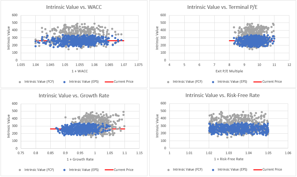
In these plots, each point represents one of the 500 intrinsic value estimates. Data points above the current price line indicate a potential combination of inputs which would suggest the stock is undervalued today. Points below the current price line indicate combinations of inputs which suggest the stock is overvalued today. In this case, as there are no clear trends in the data, the valuation seems to be generally insensitive to any of these parameters, suggesting no one input on its own is enough to drive the intrinsic value estimate. This means quite a large number of combinations could produce a valuation above the current price from a number of different inputs.

Collating these 500 points into a probability distribution yields the following:

From the sample, there is a 20% chance that the combination of inputs within the ranges specified could produce an intrinsic value below 228p in terms of EPS, or 250p in terms of free cash flow.

The most likely result (statistically, the ‘mode’) for intrinsic value, considering both an EPS and FCF/share assessment, is between 215p and 284p, and nominally around 250p. The median, i.e. the estimated intrinsic value from which there is a 50:50 chance that the ‘real’ intrinsic value is actually lower or higher, is 258p for EPS and 309p for FCF.

There is only a 20% chance that intrinsic values above ~300p can be justified, based on EPS, while a value of around 400p could possibly be justified, based on FCF/share (given my assumed range of FCF and growth rates).

At this point, let’s apply a sanity-check on the data. How likely is it that Sainsbury’s share price could drift between 200p and 300p, or even 400p? Below is the 5-year share price graph from the last 5 years from Google Finance.

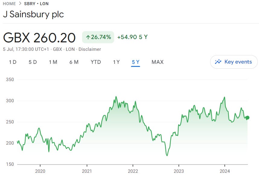
The range of 200p - 300p encompasses the majority of the share price history, with occasional periods at lower prices and very sporadic (but short-lived) breaks to above 300p. So, if you expect future performance to be similar to historic performance, that 200p - 300p range looks reasonable. But perhaps 400p is too optimistic - so perhaps some of my FCF assumptions should be reviewed, unless there is good reason to think FCF will be markedly higher in the future than it has been in the past.

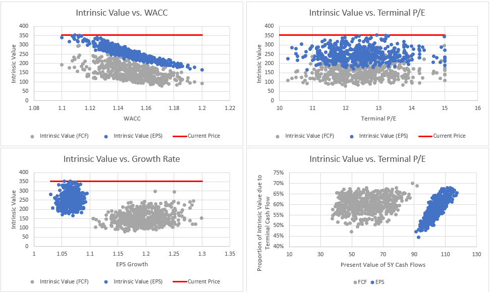
So, in the case of Sainsbury’s, the relatively low assumed growth and my relatively wide assumed ranges mean there are no obvious factors that are mostly responsible for setting the intrinsic value. Is that always the case? When I previously undertook my breakdown of intrinsic value for Rolls Royce (here), there is a very clear dependency on the cost of capital. For the input assumptions I had made at the time, justifying the then-present share price of roughly 350p, the cost of capital needed to be in the range of 10% or less and price/earnings ratio likely needed to be around 12 or higher. If you thought these assumptions were reasonable, or could even be bettered, you would likely have felt Rolls Royce justified its share price. Clearly, at 453p, the bar is markedly higher now! Or…. Rolls Royce may currently be overvalued….possibly?

This kind of insight is sufficient for me to decide on fair value, without needing to determine an estimated growth rate as in the case of a Reverse DCF.

How might Monte Carlo mislead you?

• The illusion of accuracy. Garbage in = garbage out. Just because there are lots of numbers and some relatively clever analysis going on does not mean the approach is any more fundamentally capable that other approaches to DCF analysis. It still relies on the veracity of the input data.

• Too wide ranges for inputs. It might be tempting to ‘hedge your bets’ and put wide ranges in to the inputs. But this has two consequences:

  • 1. The average value for each of the inputs might be pulled down if you assume a very low value for lower bound, compared to the assumed upper bound value. Therefore it might be easy to unintentionally build a level of conservatism into your modelling, pulling the intrinsic value down

  • 2. Wide ranges lead to large standard deviations and a lot of variation in the projected intrinsic value, obscuring the key drivers of the share price and possibly leading to a very large window of possible intrinsic values. This means it could require a very large movement from the current price to reach either high margins of safety for buying or a ‘fully valued’ position for selling. In other words, wide ranges might make it hard for value investors to find either entry or exit points if relying solely on this analysis.

• Too narrow ranges for inputs. If only small ranges for inputs are assumed, the intrinsic value will also end up in a narrow range. But if those input assumptions are ultimately shown to have been biased towards optimistic (or pessimistic) assumptions, for example if extraordinary items or a particularly beneficial and short-term macro environment have driven the performance used to set input values, and future performance deviates significantly from these assumptions, the intrinsic value will not reflect the range of possible future outcomes.

Monte Carlo or Reverse DCF?

I could generate a Monte Carlo approach based on the calculations for a reverse DCF, and maybe at some point I will, but my current Monte Carlo approach already lets me see how the growth rate contributes to the intrinsic value, given my other assumptions. So I don’t currently see what a Reverse DCF will give me over and above my Monte Carlo assessment, and therefore, I just use the ‘standard’ DCF method as the basis for my Monte Carlo analyses.

How about you? Do you use DCF, Reverse DCF or a Monte Carlo approach? Which do you find most, or least, useful?