


Valuation: My valuation sheet
Walking through my valuation sheet, available to paid subscribers

I have made the valuation sheet I use for my posts available to paid subscribers via Google Sheets, now with a Reverse DCF calculation, as I had discussed in my previous post on my Monte Carlo approach (here).
I thought I would write an article to explain how my valuation sheet works and what a paid subscriber can expect. I hope this will also act as a quick reference guide for anyone looking to use the sheet themselves.
The Layout
Fundamentally, my valuation sheet provides intrinsic valuations based on a 5-year Discounted Cash Flow (DCF) approach, coupled with a Monte Carlo analysis, as described previously. To recap, I generate a 500-point sample, selecting values randomly from pre-defined ranges for a number of input parameters used to generate an intrinsic value.
The workbook is set up in Google Sheets as follows:
A “How-To” guide, essentially the same content as in this post
A “Summary” tab, which will have the vast majority of the data and results used to generate and understand intrinsic values and the annualised growth rates required to achieve the target price.
Calculation tabs for both standard and reverse DCF approaches
A tab to collate the data used for boxplots (explained later)
I’ll now walk through how to use the sheet, using the “Summary” tab (the other tabs contain the calculations behind the summary data but are of less interest for this post).
Input Data
The DCF approach I have used is a 2-stage DCF, with a 5 year growth period, followed by a perpetual growth rate defined by the Gordon Growth Model with the Modigliani-Miller hypothesis (i.e. replace the dividend value in the Gordon Growth Model with Earnings Per Share (EPS) or Free Cash Flow Per Share (FCF/share)).
N.B. Because it is possible for the Gordon Growth Model to generate extremely large valuations when the cost of capital is very close to the risk-free rate, I have bounded the perpetual-growth element of the valuation to be within a specific price/earnings range (defined by the Terminal P/E) that would apply at the end of the DCF period.
The sheet runs two intrinsic value analyses - one using EPS and one using FCF/share. If free cash flow reflects earnings, both approaches will provide similar intrinsic values, but if the EPS and FCF, or their respective growth rates, vary significantly, then the intrinsic values for the stock could also differ wildly. In this case, it will be down to the user to choose the valuation method they believe to be most representative of the stock’s true value.
To avoid ambiguity with whether to input data as percentage points or as fractions as relative changes or as absolute growth rates, etc., I have set the sheet up specifically to take the absolute size of compounded annual growth rate (CAGR) for EPS and FCF. In other words, if you want to model a 20% - 30% CAGR for EPS, as shown below, you would put the minimum CAGR into the sheet as 1.2 and the maximum CAGR as 1.3. If you wished to model a -10% growth rate, you would enter 0.9 into the sheet.
Other inputs are the current book value of the stock, a discount factor to convert future cash flows to a present-day value (I use the Weighted Average Cost of Capital, or WACC, for this purpose) and a risk-free rate (RFR, which I usually set to be the 5-year treasury yield). As with the EPS and FCF/share CAGR inputs, I have set up WACC and RFR to also use absolute values, so a 2% risk-free rate would be inputted as 1.02.
In addition to setting ranges for minimum and maximum values to use for each parameter, at this point you can also specify what kind of distribution of inputs you want within the defined ranges. The sheet is set up to enable a uniform distribution (i.e. every value within the prescribed range is equally likely to occur), a normal distribution (it is more likely to sample values from close to the midpoint of the defined range), or a lognormal distribution (it is more likely to sample values from the lower half of the defined range).
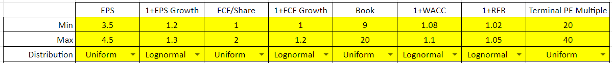
To summarise, here are all of the inputs listed:
Current EPS and EPS annualised growth rate (defined as an absolute value). To model share buybacks or share dilution over this period, the user can adjust the growth rate accordingly.
Current Free Cash Flow per share and FCF per share annualised growth rate (defined as an absolute value). As with EPS, share buybacks or dilution can be modelled by adjusting the growth rate.
Current book value. You can either put the same value in as both ‘min’ and ‘max’, which will make the analysis always use the single specified value, or you can adjust min and max to reflect nominal and tangible book values (or other values you believe are relevant to the present equity value per share). I use my own adjustments to discount inventory, intangible assets and goodwill and tax assets.
Discount Factor for adjusting future cash flows or earnings. I prefer to use a company’s Weighted Average Cost of Capital for this, and I have set the sheet up with this parameter in mind, but equally an alternative cost of equity, such as the Capital Asset Pricing Model (CAPM), or other discount factor could be used instead.
Terminal Price/Earnings - to limit the mathematical risk of large numbers being generated by the Gordon Growth Model perpetual cash flow calculation, a maximum valuation multiple is applied to cap the future price/earnings or price/free cash flow, selected at random from the range provided.
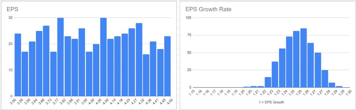
As an example of how the Monte Carlo approach then creates probability distributions from the input parameters, I have shared a screenshot of two of the distributions below. Graphical distributions for each of the input parameters are available from the “Std DCF Calculations” tab. Summary statistics on the distributions (mean, median, standard deviation and standard error) are available directly under the input data on the “Summary” tab.

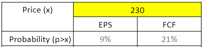
Also on the “Summary” tab is a space for you to enter your target price, such as the current price if looking to assess whether the current price represents fair value or not. Please take care to enter the price in the same currency and the same units as the earnings per share and free cash flow per share data! The sheet will then calculate the probability of the target price being a fair reflection of the intrinsic value, depending on the other inputs you have specified for each of the EPS and FCF/share analyses.
Output Data
Intrinsic Value - Standard DCF
With your assumptions entered for each of the requested parameters and for your target price, the sheet will generate distributions of intrinsic value, based on both earnings and free cash flow data, assuming a 5-year growth period. This data is generated from the 500-point Monte Carlo samples. Because the sheet uses random number generators, the specific results will change every time the sheet is used or modified, even for the same input ranges. The data table provides the price points for specific probabilities. For the example below, based on the sample data, there is an 80% chance the intrinsic value is greater than $156 based on EPS data, or $175 based on FCF/share data (the ‘P20’ point), but there is only a 9% or 21% chance that the intrinsic value is higher than the target price of $230, and the intrinsic value is most likely to be around $178, between $155 and $202.
N.B. the example below is from a different analyses to the input data shared above, in this case to show how EPS and FCF can provide similar, but slightly different, intrinsic values when EPS and FCF are specified within similar ranges.

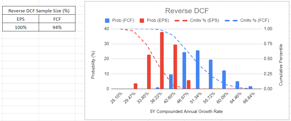
Required Growth Rate - Reverse DCF
The sheet also calculates the growth rate that would be required for each of the 500 points in the sample.
Care point - the sheet undertakes recursive calculations for the growth rate, which introduces the possibility of numerical instability. Data points that do not meet the requirements for converged solutions are rejected.
As the intrinsic value is uncertain, varying with changes in the inputs, so the required growth rate will vary depending on the specific values assumed for the inputs. Therefore, a distribution of growth rates is generated across the 500-point sample to achieve a defined target price. In the example given below, 6% of the free cash flow results have been rejected as having too large a convergence error at the end of the calculation. For the results shown in Figure 5, this company would need to exhibit a 5-year CAGR of around 40% (between 30% and 50%) to justify the target price based on EPS, and between 40% and 60% CAGR (most likely ~50% CAGR) to justify the target price based on the projected FCF/share.
Influence of the Input Parameters
Also available on the “Summary” tab, plots showing how the outputs of the Monte Carlo analyses vary with different values of the input parameters enable you to explore trends and sensitivities. In the example below, it can be seen that book value is not really an important parameter to justifying the intrinsic value and that, although it tends to be the case that a lower cost of capital can enable a higher intrinsic value (as may have been expected), the target price can be achieved (based on EPS) across most of the range of WACC considered.

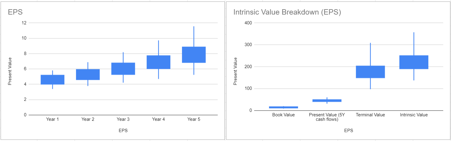
Intrinsic Value Breakdown
The last set of output plots on the “Summary” tab show a breakdown of the sources of intrinsic value from the EPS and from the FCF/share analyses. In the example below, it is obvious that the present value of future cash flows is increasing quite substantially over the 5 year growth period assumed but, despite that, the book value and the present value of the 5 years; cash flows contribute relatively little to the intrinsic value. In other words, a lot of this particular stock’s value today is derived from the perpetual growth assumed at the end of the growth period.
The Bottom Line
My valuation sheet hopefully shows how a Discounted Cash Flow can be coupled with Monte Carlo analyses to give relatively deep insights into the sources of intrinsic value, given the various uncertainties inherent in any such calculation involving speculation about the future.
I hope this proves to be a useful tool for my paid subscribers. Thank you for your continued support.